Liquid Neural Networks: Redefining AI Adaptability and Edge Computing
2026-07-16
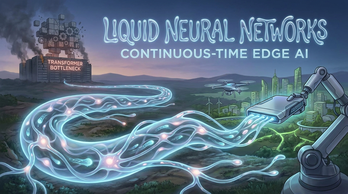
Executive Summary
The artificial intelligence landscape is colliding with the physical limits of computational scaling. While standard Transformer models continue to grow, exponentially larger models are yielding logarithmically diminishing returns; for instance, scaling a model from 7 billion to 70 billion parameters—a 10x increase in compute and memory demands—often yields fractional single-digit percentage gains on complex reasoning benchmarks [cite: 1]. Furthermore, Transformers are architecturally rigid post-training and scale poorly in memory, with standard 1-billion-parameter models requiring over 524 MB just for contextual memory at a 32,000-token sequence length [cite: 2].
Liquid Neural Networks (LNNs) represent a foundational paradigm shift away from discrete, static architectures. Inspired by the biological nervous system of the C. elegans nematode, LNNs utilize continuous-time differential equations to adapt their parameters dynamically during inference. This results in extreme parameter efficiency: an autonomous driving task can be managed by an LNN containing merely 19 neurons and 253 synapses, achieving parity with standard deep networks requiring over 100,000 neurons [cite: 1, 3]. The invention of Closed-form Continuous-time (CfC) networks has resolved the computational bottlenecks of earlier continuous models, making LNNs highly viable for production in latency-sensitive environments [cite: 4, 5, 6].
Recent breakthroughs by Liquid AI have demonstrated that the core principles of continuous-time adaptation can be hybridized to solve static text generation at scale. The introduction of Liquid Foundation Models (LFMs)—including the 1.3-billion and 3.1-billion parameter variants—proves that hybrid architectures can match Transformer benchmark accuracy while utilizing a fraction of the memory (e.g., operating a 32,000-token context in merely 192 MB of cache) [cite: 2, 7]. Consequently, while Transformers maintain supremacy in massive, cloud-based natural language processing, LNNs and their hybrid descendants are poised to dominate edge computing, autonomous robotics, and continuous time-series analysis.
The Biological Blueprint: C. elegans and the Origin of Adaptability
The genesis of Liquid Neural Networks is intrinsically linked to the biological study of Caenorhabditis elegans, a microscopic nematode worm. Despite possessing a nervous system composed of only 302 neurons, the organism exhibits remarkably complex behavioral dynamics, capable of navigation, foraging, and avoiding predators in unpredictable environments [cite: 1, 4].
Computer scientists observed that the worm's neurological efficiency does not stem from massive parallel processing or millions of synaptic connections, but from the fluid nature of the synapses themselves. In standard artificial neural networks (ANNs), a neuron passes data through a static matrix of weights using a fixed, discrete activation function, such as a ReLU (Rectified Linear Unit, a function outputting the input if positive, otherwise zero) or a Sigmoid (a mathematical function that maps input values into a smooth S-curve between 0 and 1). In contrast, biological neurons operate via continuous-time dynamics where the fundamental laws governing the neuron's response change based on the continuous stream of inputs it receives [cite: 8, 9, 10].
Translating this biological reality into code led to the creation of Liquid Time-Constant (LTC) networks. In an LTC architecture, the neural network's hidden states—which act as its memory and decision-making logic—are not fixed. If the environment becomes chaotic or noisy, the "liquid" network alters its internal wiring in real-time, effectively increasing or decreasing its temporal focus to isolate critical incoming signals and discard irrelevant noise [cite: 8, 10, 11]. This enables continuous learning without suffering from catastrophic forgetting or the loss of plasticity that plagues traditional models when exposed to out-of-distribution data [cite: 3, 11].
Deconstructing the Mechanics of Continuous-Time Neural Networks
To understand the paradigm shift LNNs represent, one must decouple from the concept of discrete time steps. Traditional Recurrent Neural Networks (RNNs), Long Short-Term Memory (LSTM) networks, and Transformers process data frame by frame or token by token [cite: 3, 12]. They expect data to arrive at predictable, uniform intervals. However, the physical world does not operate in discrete frames. Medical patient vitals, autonomous vehicle sensor readings, and financial market ticks arrive at highly irregular intervals.
Liquid Neural Networks belong to a specific class of Continuous-Time Recurrent Neural Networks (CT-RNNs). Instead of relying on static matrix multiplications, the evolution of an LNN's hidden state over time is governed by Ordinary Differential Equations (ODEs) [cite: 3, 4, 5]. An ODE is a mathematical equation that relates a continuously changing function with its derivatives over time. Think of it like observing fluid dynamics: rather than measuring the volume of water in a bucket at discrete, one-minute intervals, an ODE mathematically models the continuous, ongoing flow of water exiting a tap at any given microsecond. This continuous-time formulation grants the network native fluency in irregularly sampled time-series data [cite: 1, 3, 12].
The defining mathematical feature of a Liquid Time-Constant network is its adaptive time constant. In a standard Neural ODE, the derivative of the hidden state is defined by a neural network, but the rate at which the state decays or updates is uniform. In an LTC, the time constant itself is a function of the input. The neuron's integration window changes in real-time, allowing it to transition seamlessly between short-term rapid adaptation and long-term sustained memory [cite: 4, 13]. Importantly, the mathematics of LTCs bound both the state and the time constant to a finite range. This intrinsic mathematical boundary guarantees stability, meaning LNNs are not vulnerable to exploding gradient problems (where mathematical weight updates compound uncontrollably during training, causing the neural network to catastrophically fail) [cite: 4, 11, 13].
The Bottleneck of Numerical Solvers and the CfC Breakthrough
Despite their theoretical elegance and remarkable parameter efficiency, early Liquid Time-Constant networks faced a severe practical hurdle: computational latency during training. Because the networks were governed by continuous ODEs, evaluating the network required iterative numerical ODE solvers [cite: 4, 6, 13].
The computational complexity of these solvers varies drastically. The Euler method is a first-order solver with a local truncation error of $O(h)$; it requires only one function evaluation per step, meaning that decreasing the step size by a factor of 10 reduces the error by a factor of 10. Conversely, the Classical Runge-Kutta (RK4) method is a fourth-order solver with an error margin of $O(h^4)$, requiring four function evaluations per step. While RK4 is exponentially more accurate—decreasing the step size by a factor of 10 reduces the error by a factor of 10,000—it is computationally burdensome [cite: 14, 15]. Furthermore, stepping through continuous time requires these numerical solvers to estimate slopes over discrete slices. Because each sequential step relies on the mathematical approximation of the previous step, microscopic truncation errors accumulate. In deep networks, these compounding error bounds cause the model's temporal dynamics to drift and eventually destabilize, rendering the training of deep LNNs orders of magnitude slower than parallelized Transformers [cite: 4, 16].
The critical breakthrough that propelled LNNs into production viability was the development of the Closed-form Continuous-time (CfC) neural network. A closed-form analytical solution provides an exact mathematical formula to solve the equation directly in a single step, without requiring iterative guessing. Consider the physical analogy of calculating a car's journey: instead of adding up its incremental position second-by-second using a stopwatch and speedometer (numerical integration), a closed-form solution uses a direct formula (Distance = Rate × Time) to instantly output the exact position. By bypassing numerical ODE solvers entirely, CfC networks achieve training and inference speeds comparable to traditional discrete-time RNNs while maintaining their fluid adaptability [cite: 4, 5, 6, 17].
Architectural Synthesis: Transformers vs. Liquid Neural Networks
To accurately gauge the impact of LNNs, they must be situated alongside the reigning champions of AI architecture: Transformers and SSMs (State Space Models, architectures that compress historical data into a fixed-size mathematical state). Transformers rely on the self-attention mechanism, which maps long-range dependencies by mathematically comparing every token in a sequence to every other token. This global context comes at a brutal computational cost and creates severe KV-Cache (Key-Value Cache, memory used to store past tokens for contextual recall) bloat [cite: 4, 7, 9].
The following table provides a comprehensive comparative evaluation of the leading sequence modeling architectures using exact computational footprints for parity.
| Architectural Feature | Liquid Neural Network (CfC) | Transformer (Self-Attention) | State Space Model (e.g., Mamba) |
|---|---|---|---|
| Core Paradigm | Continuous-Time Recurrent | Discrete-Time Parallel | Discrete/Continuous Hybrid |
| Time Scaling Cost | Linear $O(N)$ [cite: 4] | Quadratic $O(N^2)$ [cite: 4, 9] | Linear $O(N)$ [cite: 4, 9] |
| Space (Memory) Scaling Complexity | Constant $O(1)$ during generation [cite: 2] | Linear $O(N)$ (KV-Cache grows per token) [cite: 2, 7] | Constant $O(1)$ during generation [cite: 2] |
| ~1B Parameter Context Memory Footprint (at 32k tokens) | ~192 MB (via hybrid LFM architectures) [cite: 2] | ~524 MB (e.g., Llama 3.2 1B) [cite: 2] | Negligible (Fixed hidden state) [cite: 2] |
| Parameter Adaptation | Dynamic post-training via fluid time constants [cite: 9, 18] | Completely Static post-training [cite: 1, 9] | Static weights (though hidden states evolve) [cite: 9] |
The downstream implications of this architectural divide are profound. Replacing power-hungry datacenter models with ultra-efficient LNNs on the edge has massive environmental and economic consequences. Datacenter Transformer training and inference consume gigawatt-hours of electricity and require massive cooling infrastructure. Transitioning to localized edge LNNs drastically reduces carbon footprints, shifts compute costs away from expensive enterprise cloud API subscriptions, and relieves strain on regional power grids [cite: 1, 19].
The Native Habitat of LNNs: Edge Computing and Autonomous Robotics
The theoretical advantages of LNNs translate into unprecedented real-world capabilities in edge artificial intelligence and autonomous control systems. In benchmark studies, an autonomous vehicle lane-keeping task was successfully managed by an LNN containing merely 19 liquid neurons and 253 synapses, drastically outperforming a conventional deep neural network requiring over 100,000 parameters [cite: 1, 3, 9].
This massive reduction in parameter count maps directly to hardware viability. On IoT (Internet of Things, interconnected physical devices embedded with computing sensors) platforms and microcontrollers, a 19-neuron LNN requires less than 1 MB of RAM. Advanced aerospace deployments, such as a Mamba-KAN-Liquid hybrid model for UAV telemetry cybersecurity, maintain a microscopic 96 MB memory footprint. On mobile SoCs (System on Chips, integrated circuits holding all essential computing components on a single substrate), 1-billion parameter models can run natively, consuming only around 719 MB of total device RAM [cite: 2, 20].
Moreover, LNNs offer drastic reductions in inference latency. In modern robotic control, standard diffusion-based policies (such as Flow Matching models) often suffer from 61 to 110 milliseconds of inference latency, creating a dangerous "inference delay" where the physical world changes before the robotic command executes [cite: 21, 22]. LNNs operate with a minimal inference pipeline, requiring roughly 20 to 250 milliseconds per batch depending on scale, but crucially executing a single forward pass without the need for iterative denoising loops, often enabling a nearly 4.8-fold latency reduction compared to heavy generative policies [cite: 20, 22, 23].
Beyond speed and size, LNNs offer critical medical and safety interpretability. Engineers can trace mathematically which specific liquid neuron responded to a sudden change in an environment. In highly regulated settings—such as analyzing irregularly sampled ECG (Electrocardiogram, measuring heart electrical activity) or EEG (Electroencephalogram, measuring brain electrical activity) readings to predict arrhythmias—this auditable, interpretable decision-making is indispensable [cite: 9, 12, 24].
Implementing Dynamic Information Flow: A Practitioner's Perspective
The transition from theoretical mathematics to practical engineering is heavily supported by the open-source community. For production-grade Liquid Neural Networks, researchers and developers utilize the ncps (Neural Circuit Policies) package [cite: 24].
- Functional Scope: The
ncpslibrary provides a native PyTorch and TensorFlow framework for deploying Liquid Time-Constant (LTC) and Closed-form Continuous-time (CfC) layers, designed explicitly for sparse recurrent networks [cite: 6, 24]. - Current Price/Cost: The package is entirely free and open-source, released under an Apache/MIT-style license suitable for commercial deployment without enterprise fees [cite: 24].
- Availability: The source code is hosted on GitHub and is easily installed via standard Python package managers (
pip install ncps) [cite: 24, 25]. - Real-World Context: The
ncpspackage is highly praised by the edge-AI community for sensor and anomaly detection on IoT hardware. Its strict anti-use case is building massive natural language generation models, as pure continuous-time networks struggle to process discrete, static text sequences efficiently at a multi-billion parameter scale [cite: 18, 25].
The following PyTorch snippet demonstrates the architecture of a continuous-state reservoir utilizing ncps mechanics.
import torch
import torch.nn as nn

class EchoStateLiquidNet(nn.Module):
 def __init__(self, input_size, reservoir_size, output_size):
 super(EchoStateLiquidNet, self).__init__()
 self.reservoir_size = reservoir_size

 # W_in: Maps incoming data into the continuous reservoir
 self.W_in = nn.Linear(input_size, reservoir_size, bias=False)

 # W_res: The dynamic hidden state connections
 self.W_res = nn.Linear(reservoir_size, reservoir_size, bias=False)

 # W_out: Extracts the final prediction from the fluid state
 self.W_out = nn.Linear(reservoir_size, output_size)

 def forward(self, input_data):
 # input_data shape: (batch_size, sequence_length, features)
 batch_size = input_data.size(0)
 seq_len = input_data.size(1)

 # Initialize the dynamic state at zero
 state = torch.zeros(batch_size, self.reservoir_size).to(input_data.device)
 outputs = []

 # Sequential processing: The network updates dynamically step-by-step
 for t in range(seq_len):
 u_t = input_data[:, t, :]

 # The fluid update: Combining new input with the persistent state
 state = torch.tanh(self.W_in(u_t) + self.W_res(state))
 outputs.append(self.W_out(state))

 return torch.stack(outputs, dim=1)
The Future Horizon: Resolving the Scaling Contradiction with LFMs
A persistent critique in the machine learning community was the inherent contradiction in scaling continuous-time physics to discrete language. If pure LNNs apply differential equations to continuous biological dynamics, how could they process static text tokens, which do not evolve continuously in physical space? Liquid AI resolved this architectural contradiction by releasing a suite of Liquid Foundation Models (LFMs), including LFM-1B (1.3 billion parameters) and LFM-3B (3.1 billion parameters) [cite: 1, 7, 18].
To overcome the strict continuous-time bottleneck for discrete text, Liquid AI entirely redesigned the structural mechanics. Rather than relying solely on pure ODEs, the LFM2 architecture utilizes a hybrid approach consisting of 16 blocks: 10 gated short convolution blocks and 6 grouped query attention blocks. By blending the adaptive state mechanics of LNNs with the compression of State Space Models and the targeted retrieval of limited attention mechanisms, Liquid AI successfully bypassed the static text barrier while preserving the $O(1)$ constant memory scaling [cite: 2, 26].
- Functional Scope: LFMs act as general-purpose generative AI models for text, vision, and time-series data, specifically optimized for edge deployment (e.g., LFM-1B on base smartphones, LFM-3B on drones) and complex reasoning (supporting up to a 32K context window) [cite: 7, 11, 26].
- Current Price/Cost: LFMs feature a unique commercial license. They are open-source and free to download, run, and fine-tune for commercial use until a company surpasses $10 million in annual revenue. Beyond that threshold, an enterprise commercial license and API costs apply [cite: 19, 27, 28].
- Availability: The models are readily accessible for direct download on Hugging Face, can be tested via the Liquid Playground, and are integrated into the LEAP (Liquid Edge AI Platform) framework [cite: 19, 29].
- Real-World Context: LFMs are the definitive choice for mobile assistants, private enterprise networks, and latency-sensitive safety systems where cloud API pricing is prohibitive. Conversely, their anti-use case remains absolute max-scale, trillion-parameter cloud NLP tasks where massive Transformer arrays (e.g., GPT-4) still dominate [cite: 19, 26].
As artificial intelligence seeps out of the datacenter and into the chaotic physical world, foundational architectures must reflect the realities of constrained hardware and continuous time. Liquid Neural Networks and their hybrid LFM successors provide the blueprint for efficient, localized machines that adapt in the moment, fundamentally challenging the assumption that intelligence requires unbounded scale.
Sources & References
- ajithp.com
- medium.com
- arxiv.org
- manifestro.io
- github.com
- arxiv.org
- liquid.ai
- codefinity.com
- theainewsdigest.com
- arxiv.org
- thenewstack.io
- ultralytics.com
- aaai.org
- libretexts.org
- medium.com
- wolfram.com
- github.com
- medium.com
- liquid.ai
- mdpi.com
- arxiv.org
- arxiv.org
- arxiv.org
- github.com
- github.com
- puter.com
- liquid.ai
- liquid.ai
- huggingface.co